Large Language Models: Theory and Practice

To use LLMs well in research you need two things: how they work, and how to use them responsibly.

Part 1 — intuition

tokens → embeddings → positional encoding → attention → Transformer → LLM

Part 2 — research practice

prompting → text analysis → literature review → validation

1. What is an LLM?

Machine Learning
   ↓
Neural Networks
   ↓
Deep Learning
   ↓
Transformer Models
   ↓
Large Language Models

• Machine learning — models that learn patterns from data
• Neural network — learns a function mapping inputs to outputs
• Deep learning — a network with many layers, each transforming the input further
• Transformer — an architecture built for sequences; its innovation is attention, letting each token weigh which other tokens matter
• LLM — a large Transformer trained on massive text, doing one simple thing: predict the next token

Neural networks

Figure: Generated by AI

Hidden layers turn the input into intermediate representations. Each node combines the previous layer, applies a nonlinearity, and passes it on. Nobody designs these patterns — the model learns them.

An LLM is the same idea with text tokens as inputs:

$$\text{features} \rightarrow \text{prediction} \qquad \text{becomes} \qquad \text{previous tokens} \rightarrow \text{next token}$$

---

How LLMs actually work

The story in six steps:

1. Text becomes tokens (chunks the model can do math on).
2. Tokens become vectors that carry meaning ("embeddings").
3. Attention lets every token weigh how much every other token matters.
4. Stack a bunch of attention layers and you have a Transformer.
5. Different kinds of Transformer (encoder vs. decoder) → different uses (BERT vs. ChatGPT).
6. Training is just "predict the next word, a lot," followed by some human-feedback polishing.

1.1 Tokens — How text becomes model input

Before anything else happens, your text is chopped into tokens — chunks of characters. Modern LLMs usually use subword tokens, not exactly words.

The model never sees letters or words directly, only these chunks. This one fact explains many things, including:

• Why models miscount letters ("how many r's in strawberry?")
• Why rare words and non-English text are handled less well
• Why API bills are measured in tokens, not words

%pip install numpy tiktoken anthropic sentence-transformers scikit-learn --quiet
import numpy as np
print("ready")

   ━━━━━━━━━━━━━━━━━━━━━━━━━━━━━━━━━━━━━━━━ 0.0/837.5 kB ? eta -:--:--
   ━━━━━━━━━━━━━━━━━━━━━━━━━━━━━━━━━━━━━━╸━ 809.0/837.5 kB 24.1 MB/s eta 0:00:01
   ━━━━━━━━━━━━━━━━━━━━━━━━━━━━━━━━━━━━━━━━ 837.5/837.5 kB 15.6 MB/s eta 0:00:00
ready

def get_tokenizer_with_ids():
    try:
        import tiktoken
        enc = tiktoken.get_encoding("cl100k_base"); enc.encode("test")
        def tokenize(s):
            ids = enc.encode(s)
            pieces = [enc.decode([i]) for i in ids]
            return list(zip(pieces, ids))
        return ("tiktoken", tokenize)
    except Exception:
        print("(tiktoken unavailable — fallback shows fake IDs)\n")
        import re
        def tokenize(s):
            pieces = re.findall(r"\s+|\w+|[^\w\s]", s)
            return [(p, hash(p) % 100000) for p in pieces]  # fake but illustrative
        return ("fallback", tokenize)

name, tokenize = get_tokenizer_with_ids()

for t in ["strawberry", "literature review", "ethnography", "café", "Central Bank", " Bank", "Bank"]:
    pairs = tokenize(t)
    print(f"\n{t!r}")
    for piece, tid in pairs:
        print(f"    {piece!r:>12}  ->  id {tid}")
print(f"\n(tokenizer: {name})")

'strawberry'
           'str'  ->  id 496
            'aw'  ->  id 675
         'berry'  ->  id 15717

'literature review'
         'liter'  ->  id 69191
         'ature'  ->  id 1598
       ' review'  ->  id 3477

'ethnography'
           'eth'  ->  id 774
             'n'  ->  id 77
       'ography'  ->  id 5814

'café'
            'ca'  ->  id 936
            'fé'  ->  id 59958

'Central Bank'
       'Central'  ->  id 44503
         ' Bank'  ->  id 8715

' Bank'
         ' Bank'  ->  id 8715

'Bank'
          'Bank'  ->  id 26913

(tokenizer: tiktoken)

Tokens are integer IDs. A tokenizer does not only split text into pieces; it also maps each piece to an integer ID. For example, "strawberry" may become something like:

[496, 675, 15717]

This sequence of IDs is what the model actually receives. The model does not directly see the word or its letters; it learns patterns from token IDs appearing in training data.

When we talk about "embeddings" in §1.2, we mean a lookup table where each token ID indexes a vector. The "vocabulary size" of a model (often 50,000–200,000) is just the number of distinct token IDs it knows about.

1.2 Embeddings — meaning becomes geometry

text → tokens → token IDs → embedding vectors

An embedding is a list of numbers representing a token:

$$\text{embedding}(\text{"bank"}) \in \mathbb{R}^{768}$$

These vectors aren't arbitrary. Training arranges them so tokens with similar meanings sit near each other — meaning becomes geometry.

Toy example

1. Hand-assign 2-D vectors. Real models learn hundreds of dimensions; we pick coordinates so we can see them.
2. Cosine similarity compares the angle between two vectors, ignoring length: 1.0 same direction · 0.0 unrelated · −1.0 opposite.
3. Print the similarity matrix — every word against every other.

emb = {
    "interview":   np.array([0.85, 0.20]),
    "ethnography": np.array([0.80, 0.30]),
    "survey":      np.array([0.70, 0.15]),
    "regression":  np.array([-0.60, 0.70]),
    "statistics":  np.array([-0.65, 0.75]),
    "tea":         np.array([0.10, -0.90]),
}
def cos(a, b): return float(a @ b / (np.linalg.norm(a)*np.linalg.norm(b)))

print("Cosine similarity (1 = same direction, 0 = unrelated, -1 = opposite):\n")
words = list(emb)
print("            " + "".join(f"{w[:10]:>12}" for w in words))
for w1 in words:
    print(f"{w1[:10]:>10}  " + "".join(f"{cos(emb[w1], emb[w2]):12.2f}" for w2 in words))
print("\n-> qualitative-methods words cluster together;")
print("   quantitative-methods words cluster together;")
print("   'tea' floats off on its own.")

Cosine similarity (1 = same direction, 0 = unrelated, -1 = opposite):

               interview  ethnograph      survey  regression  statistics         tea
 interview          1.00        0.99        1.00       -0.46       -0.46       -0.12
ethnograph          0.99        1.00        0.99       -0.34       -0.35       -0.25
    survey          1.00        0.99        1.00       -0.48       -0.48       -0.10
regression         -0.46       -0.34       -0.48        1.00        1.00       -0.83
statistics         -0.46       -0.35       -0.48        1.00        1.00       -0.82
       tea         -0.12       -0.25       -0.10       -0.83       -0.82        1.00

-> qualitative-methods words cluster together, tend to occur in very similar contexts;
   quantitative-methods words cluster together, belonging to the same conceptual area of quantitative analysis;
   'tea' floats off on its own.

Why this matters for social science

Embeddings let you measure semantic similarity between texts. A few examples:

• Cluster open-ended survey responses by theme.
• Track how a concept shifts over time in a corpus.
• Build search that understands meaning, not just keywords.

1.3 Positional encoding — adding word order

Embeddings carry meaning but not position. Order matters:

dog bites man
man bites dog

So we add a position vector:

$$x_t = \underbrace{e_t}_{\text{meaning}} + \underbrace{PE_t}_{\text{position}}$$

Same word, different position → different input. In "I sat by the bank to read; the bank had closed":

$$e_{\text{bank}} + PE_4 \;\neq\; e_{\text{bank}} + PE_9$$

Different sentences, same position → same $PE$.

Position	"Dogs bark loudly"	"Statistics inform policy"
0	$e_{\text{Dogs}} + \mathbf{PE_0}$	$e_{\text{Statistics}} + \mathbf{PE_0}$
1	$e_{\text{bark}} + \mathbf{PE_1}$	$e_{\text{inform}} + \mathbf{PE_1}$
2	$e_{\text{loudly}} + \mathbf{PE_2}$	$e_{\text{policy}} + \mathbf{PE_2}$

Think of $PE$ as row numbers in a spreadsheet — row 1 means the same thing everywhere; what changes is what sits in it.

The original Transformer used sine and cosine waves at different frequencies:

$$PE_{(pos,2i)} = \sin\!\left(\frac{pos}{10000^{2i/d}}\right), \qquad PE_{(pos,2i+1)} = \cos\!\left(\frac{pos}{10000^{2i/d}}\right)$$

Don't memorize it. The point: every position gets a unique signature. Modern models use learned positions or RoPE — same principle.

def positional_encoding(seq_len, d):     #d is how many columns total;
    pos = np.arange(seq_len)[:, None]
    i   = np.arange(d)[None, :]          #i is which column you're currently computing
    angle = pos / np.power(10000, (2*(i//2))/d)
    pe = np.where(i % 2 == 0, np.sin(angle), np.cos(angle))
    return pe

PE = positional_encoding(seq_len=40, d=64)
plt.figure(figsize=(7,3.2))
plt.imshow(PE, aspect="auto", cmap="RdBu"); plt.colorbar(shrink=0.8)
plt.xlabel("embedding dimension"); plt.ylabel("position")
plt.title("Sinusoidal positional encoding (each row = one position)"); plt.tight_layout(); plt.show()

Reading the positional encoding map

A heatmap of position vectors. With 40 rows and 64 columns, $PE \in \mathbb{R}^{40 \times 64}$: each row is one position's vector, each column an embedding dimension, each color a value.

Each column is a wave at a different speed:

• left — fast waves, red/blue speckle, distinguishes nearby positions
• right — slow waves, near-constant stripes, distinguishes far-apart positions
• middle — visibly slowing from left to right

1.4 Attention — how tokens look at each other

A word's meaning depends on the words around it:

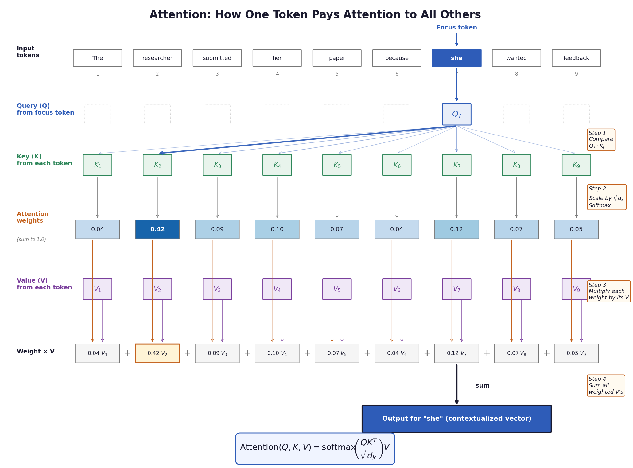
"The researcher submitted her paper because she* wanted feedback."*

Processing "she", the model must work out what it refers to. Nothing in "she" says researcher — it has to look around. Attention is that mechanism.

The three vectors

Vector	Role	Library analogy
Query (Q)	what this token is looking for	your search query
Key (K)	what this token offers	a book's title
Value (V)	what it contributes if attended to	the book's content

Each token computes its own Q, K, V through learned transformations.

$$\mathrm{Attention}(Q, K, V) = \mathrm{softmax}\!\left(\frac{QK^T}{\sqrt{d_k}}\right) V$$

• $QK^T$ — compare every query to every key
• $\sqrt{d_k}$ — scale for numerical stability
• softmax — turn scores into weights that sum to 1
• $\times V$ — weighted sum of the value vectors

Figure: Generated by AI

Walking through it, for "she" (position 7)

1 · Compare. $Q_7$ against every key $K_1 \dots K_9$ by dot product — how well does this key match what I'm looking for? Arrow thickness in the figure is the score.

2 · Normalize. Scale by $\sqrt{d_k}$, then softmax into weights summing to 1:

The	researcher	submitted	her	paper	because	she	wanted	feedback
0.04	0.42	0.09	0.10	0.07	0.04	0.12	0.07	0.05

42% of "she's" attention lands on "researcher." The pronoun is resolved — and nobody wrote that rule.

3 · Multiply, 4 · Sum. Each weight scales its value vector; the nine are added into the output for "she" — a contextualized representation, mostly shaped by researcher.

Every token does this in parallel, and all of it is learned rather than programmed.

import torch
import matplotlib.pyplot as plt
import seaborn as sns
from transformers import AutoTokenizer, AutoModel

# --------------------------------------------------
# Sentence with a clear pronoun-antecedent relation
# --------------------------------------------------
sentence = "The researcher submitted her paper because she wanted feedback."

# --------------------------------------------------
# Load tokenizer and model with attentions enabled
# --------------------------------------------------
model_name = "bert-base-uncased"
tokenizer = AutoTokenizer.from_pretrained(model_name)
model = AutoModel.from_pretrained(model_name, output_attentions=True)
model.eval()

# --------------------------------------------------
# Tokenize
# --------------------------------------------------
inputs = tokenizer(sentence, return_tensors="pt")
tokens = tokenizer.convert_ids_to_tokens(inputs["input_ids"][0])

# --------------------------------------------------
# Forward pass
# attentions: tuple of length num_layers
# each element shape = (batch, num_heads, seq_len, seq_len)
# --------------------------------------------------
with torch.no_grad():
    outputs = model(**inputs)

attentions = outputs.attentions  # tuple: one tensor per layer

# --------------------------------------------------
# Helper: find token indices
# We use exact token matching after lowercasing/tokenization
# --------------------------------------------------
def find_token_indices(tokens, target):
    return [i for i, tok in enumerate(tokens) if tok == target]

print("Tokens:")
for i, tok in enumerate(tokens):
    print(i, tok)

# For this sentence in bert-base-uncased:
# expected tokens include:
# [CLS], the, researcher, submitted, her, paper, because, she, wanted, feedback, ., [SEP]

researcher_indices = find_token_indices(tokens, "researcher")
she_indices = find_token_indices(tokens, "she")

if len(researcher_indices) == 0 or len(she_indices) == 0:
    raise ValueError("Could not find 'researcher' or 'she' in the tokenized sentence.")

researcher_idx = researcher_indices[0]
she_idx = she_indices[0]

print("\nChosen indices:")
print("researcher_idx =", researcher_idx, "token =", tokens[researcher_idx])
print("she_idx        =", she_idx, "token =", tokens[she_idx])

# --------------------------------------------------
# Find the layer/head where attention from "she" to
# "researcher" is largest
# --------------------------------------------------
best_layer = None
best_head = None
best_score = -1.0

num_layers = len(attentions)
num_heads = attentions[0].shape[1]

for layer in range(num_layers):
    # shape: (num_heads, seq_len, seq_len)
    attn = attentions[layer][0]
    for head in range(num_heads):
        score = attn[head, she_idx, researcher_idx].item()
        if score > best_score:
            best_score = score
            best_layer = layer
            best_head = head

print(f"\nBest layer/head for she -> researcher: layer={best_layer}, head={best_head}, attention={best_score:.4f}")

# --------------------------------------------------
# Extract the best attention matrix
# --------------------------------------------------
best_attn = attentions[best_layer][0, best_head].cpu().numpy()

# --------------------------------------------------
# Plot full heatmap
# Rows = querying token
# Cols = attended-to token
# --------------------------------------------------
plt.figure(figsize=(10, 8))
ax = sns.heatmap(
    best_attn,
    xticklabels=tokens,
    yticklabels=tokens,
    cmap="Blues",
    cbar=True,
    square=True
)

plt.title(
    f"BERT Self-Attention Heatmap\nLayer {best_layer+1}, Head {best_head+1}\n"
    f"(selected because 'she' attends strongly to 'researcher')"
)
plt.xlabel("Key / attended-to token")
plt.ylabel("Query token")
plt.xticks(rotation=45, ha="right")
plt.yticks(rotation=0)

# Highlight the cell (she -> researcher)
ax.add_patch(plt.Rectangle((researcher_idx, she_idx), 1, 1, fill=False, edgecolor="red", lw=3))

plt.tight_layout()
plt.show()

# --------------------------------------------------
# Also plot just the attention row for "she"
# --------------------------------------------------
she_row = best_attn[she_idx]

plt.figure(figsize=(10, 3))
sns.heatmap(
    she_row.reshape(1, -1),
    annot=True,
    fmt=".2f",
    cmap="Blues",
    xticklabels=tokens,
    yticklabels=[f"query = '{tokens[she_idx]}'"]
)
plt.title(
    f"Attention weights from 'she' to all tokens\n"
    f"Layer {best_layer+1}, Head {best_head+1}"
)
plt.xlabel("Attended-to token")
plt.ylabel("")
plt.xticks(rotation=45, ha="right")
plt.tight_layout()
plt.show()

/usr/local/lib/python3.12/dist-packages/huggingface_hub/utils/_auth.py:112: UserWarning: 
The secret `HF_TOKEN` does not exist in your Colab secrets.
To authenticate with the Hugging Face Hub, create a token in your settings tab (https://huggingface.co/settings/tokens), set it as secret in your Google Colab and restart your session.
You will be able to reuse this secret in all of your notebooks.
Please note that authentication is recommended but still optional to access public models or datasets.
  warnings.warn(
Warning: You are sending unauthenticated requests to the HF Hub. Please set a HF_TOKEN to enable higher rate limits and faster downloads.
WARNING:huggingface_hub.utils._http:Warning: You are sending unauthenticated requests to the HF Hub. Please set a HF_TOKEN to enable higher rate limits and faster downloads.

BertModel LOAD REPORT from: bert-base-uncased
Key                                        | Status     |  | 
-------------------------------------------+------------+--+-
cls.predictions.transform.LayerNorm.weight | UNEXPECTED |  | 
cls.predictions.bias                       | UNEXPECTED |  | 
cls.seq_relationship.weight                | UNEXPECTED |  | 
cls.predictions.transform.dense.weight     | UNEXPECTED |  | 
cls.predictions.transform.dense.bias       | UNEXPECTED |  | 
cls.predictions.transform.LayerNorm.bias   | UNEXPECTED |  | 
cls.seq_relationship.bias                  | UNEXPECTED |  | 

Notes:
- UNEXPECTED	:can be ignored when loading from different task/architecture; not ok if you expect identical arch.

Tokens:
0 [CLS]
1 the
2 researcher
3 submitted
4 her
5 paper
6 because
7 she
8 wanted
9 feedback
10 .
11 [SEP]

Chosen indices:
researcher_idx = 2 token = researcher
she_idx        = 7 token = she

Best layer/head for she -> researcher: layer=8, head=10, attention=0.6265

Interpreting the Heatmap

This figure shows real self-attention weights from a pretrained BERT model.

• Each row is the query token.
• Each column is the token being attended to.
• Darker color means stronger attention.

We selected the layer and head where the token "she" places the strongest attention on "researcher".

So if the cell at row she and column researcher is dark, that means:

when representing "she", this attention head uses information from "researcher".

This gives a concrete example of how attention can help connect a pronoun to its antecedent.

1.5 Multi-Head Attention

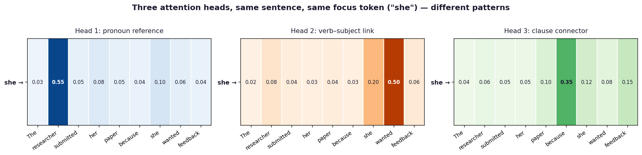
In §1.4 we walked through one attention computation. Real models run many in parallel in every layer — typically 8 to 96 of them. Each one is called an attention head.

Figure: Generated by AI

Each head learns its own notion of "what's relevant." For the same focus token ("she"), Head 1 catches the pronoun's referent (researcher), Head 2 catches the verb it controls (wanted), Head 3 catches the clause-connector (because). All run in parallel, and the model combines them.

One head sees one kind of relationship. Many heads, working in parallel, capture many at once.

1.6 From attention to Transformer blocks

Figure: the encoder stack from Vaswani et al. (2017), "Attention Is All You Need"

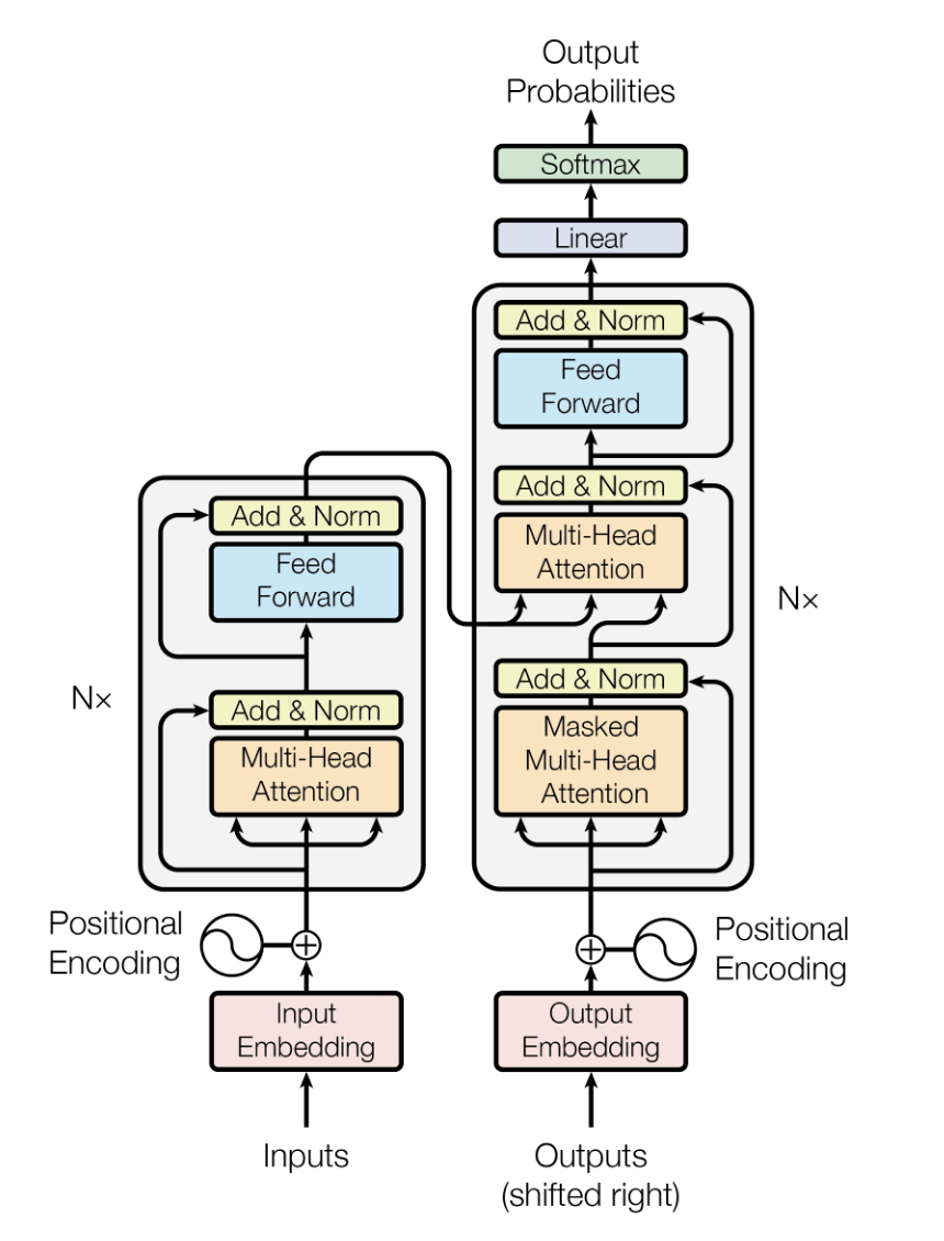
The encoder block

Bottom to top:

1. Input embedding — tokens to vectors (§1.2)
2. Positional encoding — word order (§1.3)
3. Multi-head self-attention — every token weighs every other (§1.4)
4. Add & Norm — add keeps the original input and layers changes on top, like editing rather than rewriting; norm rescales values into a tidy range. This is what lets 12, 24, or 96 blocks stack without breaking.
5. Feed forward — a small network applied to each token independently
6. Add & Norm again

N× means the block repeats — 6 in the original paper, dozens today. Each layer's output feeds the next.

What it's for: every token sees every other, so the encoder is built for understanding. Output is one context-enriched vector per token. This is BERT — classification, embeddings, similarity; not generation.

The decoder block

Bottom to top:

1. Output embedding — the tokens generated so far
2. Positional encoding
3. Masked multi-head self-attention — each token sees only earlier tokens; the mask hides the future
4. Add & Norm
5. Multi-head cross-attention — new: decoder tokens attend to the encoder's output, which is how the input sentence reaches the output sentence
6. Add & Norm
7. Feed forward
8. Add & Norm

What it's for: seeing only the past is what makes generation possible, one token at a time. Cross-attention lets it condition on something else, as in translation. GPT and ChatGPT are decoder-only — masked self-attention kept, cross-attention dropped since there's no encoder.

Why the mask matters. Without it, position 3 could peek at position 5 and next-token prediction would be trivial. The mask enforces the same rule at training time and generation time.

mask = np.triu(np.ones((T, T)), k=1).astype(bool)   # True above the diagonal = future
masked_scores = scores.copy(); masked_scores[mask] = -np.inf
causal_weights = softmax(masked_scores)
print("causal weights (note the upper triangle is 0):\n", causal_weights)

causal weights (note the upper triangle is 0):
 [[1.   0.   0.   0.   0.  ]
 [0.   1.   0.   0.   0.  ]
 [0.46 0.06 0.47 0.   0.  ]
 [0.16 0.01 0.21 0.62 0.  ]
 [0.   0.99 0.   0.   0.01]]

1.5 Why BERT ≠ ChatGPT

BERT and ChatGPT use the same building blocks — they just keep different parts.

	BERT	ChatGPT / Claude / GPT
Uses...	encoder only	decoder only
Each token sees...	every other token (both directions)	only tokens before it
Trained to...	fill in blanked-out words	predict the next word
Best for...	understanding text	generating text
Research uses	classification, embeddings, similarity	drafting, summarizing, synthesis

1.6 How LLMs are trained

Stage 1 · Pretraining. Enormous amounts of text, one task: predict the next word, trillions of times. Getting good at it forces the model to absorb grammar, facts, reasoning, and style as a side effect.

This is the source of both the magic and the trouble:

• magic — fluency, broad knowledge, following complex instructions
• trouble — the reward is for plausible next words, not true ones. That is the structural root of hallucination: an invented citation is a pattern that looks right.

Stage 2 · Post-training. Humans rate which of two responses is better and the model is tuned toward the preferred ones (RLHF and relatives). This creates the "helpful assistant" personality — along with sycophancy, over-refusal, and the hedged chatbot tone.

Why this matters for research

• Hallucination is structural, not a bug. No prompt fully removes it. Verify anything factual.
• Models change silently. Pin the model version in your methods section.
• "Helpfulness" reflects the provider's raters, which shapes what the model will engage with.

Part 2 — Using LLMs in your research

2.1 LLM or traditional method?

The first question isn't how do I use an LLM — it's should I. For many text-as-data tasks, traditional methods are cheaper, more transparent, and easier to reproduce.

Traditional methods win

Task	Use	Why
Tone across many documents	Dictionaries (Loughran-McDonald, BBD)	field standard, free, reproducible
Topics in a large corpus	Topic models (LDA, BERTopic)	purpose-built and defensible
Classify thousands of documents	Fine-tuned BERT	cheaper and more reproducible at scale

LLMs win

Task	Why
Nuanced tone in a small set of texts	handles context, hedging, sarcasm
Structured extraction from messy text	works zero-shot, no training data
Summarizing or comparing a few papers	what they're genuinely best at

Neither — recalling a citation, statistic, or fact. Use Google Scholar, FRED, your library. LLMs fabricate these.

Two principles

1. Match the tool to the task and the scale. For 100,000 documents on a fixed schema, BERT or even TF-IDF is cheaper, faster, more reproducible.
2. Traditional methods aren't obsolete. "We used the Loughran-McDonald lexicon" is easier to publish than "we used GPT-4 in March 2025."

2.2 Calling an API, and one prompting principle

How you prompt is a methodological choice. Prompts should be specific, reproducible (saved verbatim, like a survey instrument), and reported.

Why the API, not the chat window

An API lets your code talk to a model running on someone else's machine: you send text, you get an answer back.

	Chat (chatgpt.com)	API (in code)
200 documents	paste 200 times	one for loop
Reproducible?	no record of the exact prompt	yes — the code is the record
Feeds pandas, regressions, plots?	copy-paste	output flows straight in

%pip install google-generativeai --quiet

import os
import google.generativeai as genai

# Paste your NEW key (after revoking the old one) here:
genai.configure(api_key="Your API Key")

MODEL = "gemini-3.1-flash-lite"

def ask(prompt, system=None, temperature=0.0, max_tokens=1024):
    model = genai.GenerativeModel(MODEL, system_instruction=system)
    response = model.generate_content(
        prompt,
        generation_config={"temperature": temperature, "max_output_tokens": max_tokens},
    )
    return response.text

print(ask("Say hello in one word."))

/usr/local/lib/python3.12/dist-packages/google/colab/_import_hooks/_hook_injector.py:55: FutureWarning: 

All support for the `google.generativeai` package has ended. It will no longer be receiving 
updates or bug fixes. Please switch to the `google.genai` package as soon as possible.
See README for more details:

https://github.com/google-gemini/deprecated-generative-ai-python/blob/main/README.md

  loader.exec_module(module)

Hello.

Two settings that matter

• system — sets the role: "You are a careful research assistant for an Econ project."
• temperature — randomness. 0 is deterministic and right for analysis; higher is for brainstorming, not measurement.

Keep temperature=0. Variation across runs is variance you didn't intend.

The principle: ground claims in the source text

Make the model quote the input it's relying on. If it can't point to where a claim comes from, the claim is probably hallucinated. Compare these two prompts on the same input:

text = ("The policy was announced in March 2023 and applied to all departments. "
        "Most staff welcomed it, but some senior managers raised concerns about costs.")

# Ungrounded
print("--- Ungrounded prompt ---")
print(ask(f"What does this excerpt say? {text}"))

print("\n--- Grounded prompt ---")
print(ask(
    f"From the excerpt below, list the key claims. For EACH claim, quote the "
    f"exact span of text from the excerpt that supports it. If a claim is not "
    f"directly supported, say 'NOT IN TEXT'.\n\nExcerpt: {text}"
))

--- Ungrounded prompt ---
This excerpt explains three main points regarding a specific policy:

*   **Timeline:** It was introduced in March 2023.
*   **Scope:** It affected every department within the organization.
*   **Reception:** While the general staff was largely in favor of the policy, some members of senior management were worried about the financial impact.

--- Grounded prompt ---
Here are the key claims from the excerpt:

**Claim 1: The policy was announced in March 2023.**
*   **Supporting text:** "The policy was announced in March 2023"

**Claim 2: The policy applied to every department.**
*   **Supporting text:** "applied to all departments."

**Claim 3: The majority of staff reacted positively to the policy.**
*   **Supporting text:** "Most staff welcomed it"

**Claim 4: Some senior managers were worried about the financial implications.**
*   **Supporting text:** "some senior managers raised concerns about costs."

The grounded version forces the model to point at evidence, which makes hallucination immediately visible.

Treat prompts as research artifacts

• save every prompt with your code and data
• pin the model version — gemini-2.0-flash, not "Gemini"
• temperature=0 for analysis
• robustness check — try 2–3 paraphrases; if results move meaningfully, that's a finding about your measurement

2.3 Econ demo — scoring FOMC hawkishness

FOMC statements are short press releases issued after each policy meeting (eight a year) announcing the rate decision and the Committee's read of the economy. They are short, formal, and intensely scrutinized.

Scoring them hawkish (toward tighter policy) or dovish (toward easier) is a real research task with a dictionary-based literature behind it — Hansen et al., Transparency and Deliberation; Apel & Grimaldi, The information content of central bank minutes.

Task: score two real statements 1–5, hawkish to dovish, with justification grounded in the text.

fomc_2024_03 = """\
Recent indicators suggest that economic activity has been expanding at a solid pace.
Job gains have remained strong, and the unemployment rate has remained low. Inflation
has eased over the past year but remains elevated.

The Committee seeks to achieve maximum employment and inflation at the rate of 2
percent over the longer run. The Committee judges that the risks to achieving its
employment and inflation goals are moving into better balance. The economic outlook
is uncertain, and the Committee remains highly attentive to inflation risks.

In support of its goals, the Committee decided to maintain the target range for the
federal funds rate at 5-1/4 to 5-1/2 percent.
"""

fomc_2020_03 = """\
The Federal Reserve is committed to use its full range of tools to support the U.S.
economy in this challenging time and thereby promote its maximum employment and
price stability goals.

The Federal Open Market Committee is taking further actions to support the flow of
credit to households and businesses by addressing strains in the markets for Treasury
securities and agency mortgage-backed securities. The Federal Reserve will continue
to purchase Treasury securities and agency mortgage-backed securities in the amounts
needed to support smooth market functioning and effective transmission of monetary
policy to broader financial conditions.
"""

print("Two real FOMC excerpts loaded. Both are public domain (U.S. government works).")
print(f"\n2024-03: {len(fomc_2024_03)} chars")
print(f"2020-03: {len(fomc_2020_03)} chars")

Two real FOMC excerpts loaded. Both are public domain (U.S. government works).

2024-03: 678 chars
2020-03: 649 chars

Pause: predict before running

Before we run the model, look at both excerpts. Which one would you score more hawkish? Which more dovish? Make a prediction — we'll see if the model agrees.

(The 2024 statement was during the inflation-fighting period; rates were held at 5.25-5.50%. The 2020 statement is from the emergency COVID response — the Fed was easing aggressively. So we'd expect: 2024 = more hawkish, 2020 = clearly dovish.)

The prompt

prompt_template = """\
You are analyzing FOMC statements for tone. On a scale of 1 to 5:
- 1 = strongly DOVISH (committed to easing/stimulus)
- 2 = leaning dovish
- 3 = neutral
- 4 = leaning hawkish
- 5 = strongly HAWKISH (committed to tightening/inflation-fighting)

For the statement below, return a JSON object with these keys:
- "score": integer from 1 to 5
- "stance": one of "dovish", "leaning dovish", "neutral", "leaning hawkish", "hawkish"
- "evidence": a list of 2-3 SHORT direct quotes from the statement that justify the score
- "uncertainty": one sentence on what could make the score ambiguous

Return ONLY the JSON object, no other text.

Statement:
\"\"\"{text}\"\"\"
"""

import json
print("=== March 2024 ===")
raw_2024 = ask(prompt_template.format(text=fomc_2024_03))
print(raw_2024)

# Try to parse — may fail occasionally; that's a real reliability lesson
try:
    result_2024 = json.loads(raw_2024.strip().strip("`").replace("json\n", ""))
    print(f"\nParsed score: {result_2024['score']} ({result_2024['stance']})")
except Exception as e:
    print(f"\nParse failed: {e}")

=== March 2024 ===
{
  "score": 3,
  "stance": "neutral",
  "evidence": [
    "risks to achieving its employment and inflation goals are moving into better balance",
    "remains highly attentive to inflation risks",
    "maintain the target range for the federal funds rate"
  ],
  "uncertainty": "The balance between acknowledging that inflation has eased and the continued emphasis on being 'highly attentive' to inflation risks creates a tension between a pivot toward easing and a commitment to maintaining current restrictive levels."
}

Parsed score: 3 (neutral)

print("=== March 2020 ===")
raw_2020 = ask(prompt_template.format(text=fomc_2020_03))
print(raw_2020)

try:
    result_2020 = json.loads(raw_2020.strip().strip("`").replace("json\n", ""))
    print(f"\nParsed score: {result_2020['score']} ({result_2020['stance']})")
except Exception as e:
    print(f"\nParse failed: {e}")

=== March 2020 ===
{
  "score": 1,
  "stance": "dovish",
  "evidence": [
    "committed to use its full range of tools to support the U.S. economy",
    "taking further actions to support the flow of credit",
    "continue to purchase Treasury securities and agency mortgage-backed securities"
  ],
  "uncertainty": "The statement focuses on market functioning and liquidity rather than explicit interest rate policy, which could be interpreted as a technical intervention rather than a broad monetary easing stance."
}

Parsed score: 1 (dovish)

Is this score reasonable?

The model said 3 (neutral); most Econ readers would say 4 (leaning hawkish). The evidence quotes are right — the context is missing.

What the model sees	What an Econ student knows
"maintain rate at 5.25–5.50%"	the highest rate in 23 years — holding it is hawkish
"risks moving into better balance" + "highly attentive to inflation risks"	the press called this a "hawkish hold"
the statement in isolation	the statement within the cycle

Three lessons:

1. LLMs read text, not context. It doesn't know the rate is historically high or how the previous 11 statements read.
2. "Neutral" compared to what? It conflates level with direction.
3. This is why validation matters. At scale this bias pulls scores toward the middle — only visible if you hand-code a sample.

The lesson isn't that the model was right or wrong. It gave a defensible but incomplete answer — and a real workflow would catch that.

# A slightly different prompt — same task, different framing
prompt_v2 = """\
Rate the monetary policy stance of this FOMC statement.

Scale: 1 (very dovish, expansionary) to 5 (very hawkish, contractionary).

Return JSON: {{"score": int, "stance": str, "evidence": [quotes], "uncertainty": str}}

Text: {text}
"""

raw_2024_v2 = ask(prompt_v2.format(text=fomc_2024_03))
print("=== 2024-03 with paraphrased prompt ===")
print(raw_2024_v2)

=== 2024-03 with paraphrased prompt ===
```json
{
  "score": 4,
  "stance": "Hawkish",
  "evidence": [
    "Inflation... remains elevated.",
    "The Committee remains highly attentive to inflation risks.",
    "the Committee decided to maintain the target range for the federal funds rate at 5-1/4 to 5-1/2 percent."
  ],
  "uncertainty": "Low. The statement maintains a restrictive interest rate level while explicitly highlighting that inflation remains above the 2% target and that the Committee remains 'highly attentive' to those risks, signaling a 'higher for longer' approach."
}
```

What's next: validation at scale

What we did here is a single example. For a publishable analysis, you'd:

1. Hand-score a sample of ~50 statements yourself (or with a co-author).
2. Have the LLM score the same sample with the same prompt.
3. Compute agreement (e.g., weighted Cohen's κ across the 1-5 scale).
4. If agreement is good, scale to the full corpus; report agreement in your paper.

This is how LLM-coded data gets from "the model said so" to a defensible measurement procedure.

2.4 Literature Review

LLMs are useful for lit review in one specific way and dangerous in another.

✅ Safe: summarizing, comparing, and synthesizing text you provide. ❌ Dangerous: asking the LLM to recall citations from memory. It will confidently invent papers that don't exist.

The dangerous use (demo)

print(ask(
    "List three peer-reviewed papers (authors, year, title) on measuring hawkishness "
    "of FOMC statements using text analysis."
))
print("\n⚠️  TREAT AS UNVERIFIED.")
print("    Confirm every citation in Google Scholar, JSTOR, or NBER before using.")
print("    Authors, years, titles, AND journal names may all be plausibly fabricated.")

Measuring the "hawkishness" or "dovishness" of Federal Open Market Committee (FOMC) statements using natural language processing and computational linguistics has become a standard approach in empirical macroeconomics.

Here are three influential peer-reviewed papers that utilize text analysis to quantify the tone of FOMC communications:

### 1. The "Hawkish-Dovish" Dictionary Approach
*   **Authors:** Lucca, D. O., & Trebbi, F.
*   **Year:** 2009
*   **Title:** "Measuring Central Bank Communication: An Automated Approach with Application to FOMC Statements"
*   **Journal:** *Journal of Monetary Economics*
*   **Summary:** This paper is a foundational study in the field. The authors develop a methodology to measure the "hawkishness" of FOMC statements by constructing a dictionary of words associated with inflation-fighting (hawkish) versus growth-supporting (dovish) stances. They demonstrate that these automated measures correlate strongly with market reactions and policy shifts.

### 2. Sentiment Analysis and Market Impact
*   **Authors:** Hansen, S., McMahon, M., & Prat, A.
*   **Year:** 2018
*   **Title:** "Transparency and Deliberation within the FOMC: A Computational Linguistics Approach"
*   **Journal:** *The Quarterly Journal of Economics*
*   **Summary:** While this paper focuses heavily on the internal deliberation process (transcripts), it is widely cited for its sophisticated use of Latent Dirichlet Allocation (LDA) and other machine learning techniques to map the evolution of FOMC policy preferences. It provides a rigorous framework for identifying how specific topics and tones in central bank communication influence financial markets.

### 3. Measuring Policy Uncertainty and Tone
*   **Authors:** Shapiro, A. H., & Wilson, D. J.
*   **Year:** 2019
*   **Title:** "Taking the Fed at Its Word: A New Approach to Estimating Central Bank Objectives Using Text Analysis"
*   **Journal:** *Journal of Monetary Economics*
*   **Summary:** The authors introduce a new measure of the Fed’s policy stance by analyzing the text of FOMC statements. They use a "bag-of-words" approach to create a "Fed sentiment index." Their research is particularly notable for showing that their text-based measure of hawkishness is a better predictor of future interest rate changes than traditional Taylor-rule-based models.

⚠️  TREAT AS UNVERIFIED.
    Confirm every citation in Google Scholar, JSTOR, or NBER before using.
    Authors, years, titles, AND journal names may all be plausibly fabricated.

Why this happens (§1.6): the model was trained to produce plausible text, not true text. [Hansen & Smith, 2019, "Measuring FOMC Stance," JME] is a pattern it has seen thousands of times, and it will generate look-alikes whether or not the paper exists.

The safe workflow

1. You gather the papers — Google Scholar, NBER, RePEc, your library
2. You paste the abstracts or relevant sections into the prompt
3. The model summarizes, compares, and organizes the text you supplied

# Synthesizing across abstracts YOU provide is safe
abstracts = {
    "Hansen et al. (2018) QJE": "Text analysis of FOMC transcripts shows greater "
        "transparency leads to more disciplined deliberation but also conformity in "
        "individual positions.",
    "Apel & Grimaldi (2014) IJCB": "A novel dictionary-based measure of Riksbank "
        "minutes' tone predicts policy decisions one quarter ahead.",
    "Cieslak & Schrimpf (2019) JIE": "Decomposes high-frequency market reactions to "
        "FOMC announcements into monetary policy and information components.",
}

print(ask(
    "Synthesize these three abstracts in 3 sentences. Where do they agree? "
    "Where do their methods or findings differ?\n\n" +
    "\n".join(f"[{k}] {v}" for k, v in abstracts.items())
))

These three studies collectively demonstrate that central bank communication—whether through transcripts, minutes, or policy announcements—serves as a critical, quantifiable driver of both internal deliberation and external market expectations. While they agree that linguistic and high-frequency data provide significant predictive power regarding monetary policy, they differ in their focus: Hansen et al. examine the internal behavioral consequences of transparency on committee members, Apel and Grimaldi utilize dictionary-based sentiment analysis to forecast future policy, and Cieslak and Schrimpf isolate the specific market-moving components of policy announcements. Ultimately, the research diverges by shifting the analytical lens from the internal dynamics of committee conformity to the external predictive utility of tone and the structural decomposition of market reactions.

The verification rule

For any factual claim the LLM produces — citation, statistic, historical date, name — assume it's wrong until you've checked it. The cost of one fabricated citation in a published paper is much higher than the cost of verifying ten real ones.

One-line takeaway: LLMs are excellent at processing text you give them and unreliable at recalling specific facts. Build your workflow around that asymmetry.

---

Wrap-up

LLMs turn text into tokens, tokens into vectors, and use attention to connect information across a sequence. Stack attention layers and you have a Transformer. Train it to predict the next token, then refine it to follow instructions.

Use an LLM when the task needs context and flexible language understanding. Use traditional methods when it's simple, large-scale, or must be strongly reproducible.

Five takeaways

1. LLMs hallucinate. Verify every fact, citation, and statistic.
2. Prompts are research instruments. Save the exact prompt, model name, settings, and date.
3. Validation is not optional. Compare against a human-coded sample.
4. Traditional methods still matter. Dictionaries, topic models, and classifiers often win.
5. LLMs are assistants, not authorities. Interpretation stays with the researcher.

Thank you for coming, and good luck with your research.