High-Dimensional Data: From Factor Models to Deep Learning

Lusha Xu · UC Riverside · April 2026

The question: with many economic indicators, how do we extract signal to forecast GDP growth, inflation, or unemployment?

Three strategies for high-dimensional prediction:

strategy	method
compression — summarize many predictors into a few components	PCA / factor models
supervised compression — components built with the target in mind	PLS
selection — keep only what matters	Lasso
representation learning — let the model find nonlinear structure	neural networks

1. Why high dimensions are hard

• overfitting — the model fits noise instead of signal
• multicollinearity — macro variables move together and repeat information
• instability — OLS coefficients swing with correlated predictors
• interpretation — hundreds of coefficients hide what matters
• noise accumulation — irrelevant variables actively hurt

The problem is a balance: accuracy, interpretability, stability, feasibility.

The forecasting problem

Predict $y_{t+h}$ from a large predictor vector $X_t$.

Macro forecasting collects many indicators — unemployment, industrial production, payrolls, inflation, housing, sentiment — and they are not independent. They move together because a few broad forces drive them: the business cycle, financial conditions, inflation pressure.

Those hidden forces are latent factors: unobserved variables that influence many observed ones at once. When the economy weakens we see unemployment rise, production fall, sentiment drop, payroll growth slow — one force, many symptoms.

That co-movement is the whole intuition behind factor models and PCA: summarize the dataset with a few components instead of modeling every predictor separately.

In our simulation

Three persistent latent factors follow AR(1):

$$f_t = A f_{t-1} + u_t, \qquad f_t \in \mathbb{R}^3$$

60 observed indicators load on them:

$$X_t = \Lambda f_t + e_t$$

and the target depends on its own lag plus the factors, with one nonlinear term:

$$y_t = \phi y_{t-1} + (1-\phi)\left(1.5 f_{1t} - 1.0 f_{2t} + 0.7 f_{3t} + 0.4 f_{1t}^2\right) + \varepsilon_t$$

# ==================================================
# Imports
# ==================================================
import numpy as np
import pandas as pd
import matplotlib.pyplot as plt

from sklearn.pipeline import Pipeline
from sklearn.preprocessing import StandardScaler
from sklearn.linear_model import LinearRegression, LassoCV
from sklearn.decomposition import PCA
from sklearn.cross_decomposition import PLSRegression
from sklearn.neural_network import MLPRegressor
from sklearn.metrics import mean_squared_error, mean_absolute_error, r2_score
from sklearn.model_selection import TimeSeriesSplit

np.random.seed(42)

n_obs = 240          # e.g. 240 months
n_features = 60      # many predictors
n_factors_true = 3   # latent macro forces

# Generate AR(1) latent factors with persistence
ar_coeffs = [0.85, 0.7, 0.75]  # persistence parameters for each factor
F = np.zeros((n_obs, n_factors_true))

# Initialize
F[0, :] = np.random.normal(size=n_factors_true)

# Generate factors with temporal structure
for t in range(1, n_obs):
    for j in range(n_factors_true):
        F[t, j] = ar_coeffs[j] * F[t-1, j] + np.random.normal(scale=0.5)

# Factor loadings (how indicators load on factors)
loadings = np.random.normal(size=(n_features, n_factors_true))

# Generate observed predictors
X = F @ loadings.T + 0.3 * np.random.normal(size=(n_obs, n_features))

# Generate target with temporal structure
y = np.zeros(n_obs)
y[0] = (
    1.5 * F[0, 0]
    - 1.0 * F[0, 1]
    + 0.7 * F[0, 2]
    + 0.4 * (F[0, 0] ** 2)
    + 0.3 * np.random.normal()
)

# Add AR component to y itself (common in macro data)
y_ar_coeff = 0.4
for t in range(1, n_obs):
    y[t] = (
        y_ar_coeff * y[t-1] +  # AR(1) component
        (1 - y_ar_coeff) * (  # Factor-based component
            1.5 * F[t, 0]
            - 1.0 * F[t, 1]
            + 0.7 * F[t, 2]
            + 0.4 * (F[t, 0] ** 2)
        )
        + 0.3 * np.random.normal()
    )

# Create DataFrame
columns = [f"indicator_{i+1}" for i in range(n_features)]
df = pd.DataFrame(X, columns=columns)
df["target"] = y

print("Data shape:", df.shape)
df.head()

Data shape: (240, 61)

	indicator_1	indicator_2	indicator_3	indicator_4	indicator_5	indicator_6	indicator_7	indicator_8	indicator_9	indicator_10	...	indicator_52	indicator_53	indicator_54	indicator_55	indicator_56	indicator_57	indicator_58	indicator_59	indicator_60	target
0	-0.373258	0.108400	-0.379874	-0.663819	1.162093	0.849755	-0.913256	-0.308419	0.672085	-0.552760	...	0.909448	-0.674145	0.330199	0.029526	0.939029	0.774327	0.998852	0.659534	-0.488750	0.706071
1	0.425835	1.174188	-0.192566	-1.111203	1.199902	1.299020	0.872880	-0.831137	0.824786	-1.711249	...	-0.137204	-0.044044	0.463827	-0.030465	1.988011	0.569147	0.658302	1.339637	-0.258311	2.293618
2	0.253053	1.194918	0.084581	-0.750027	0.895967	1.080551	3.162664	-2.406943	0.951622	-1.865215	...	-1.102234	-0.854781	2.318338	-0.307199	3.289769	0.887443	1.080990	3.077092	0.766734	3.341299
3	0.836547	1.256853	0.021823	-0.592253	0.756693	0.763173	3.605191	-2.191473	0.864514	-1.091846	...	-1.546805	-0.458274	2.207824	-1.161420	3.641782	1.178025	0.235568	2.653538	0.556809	3.602536
4	3.502123	1.653272	0.183452	-0.450742	1.287820	-0.469162	3.264822	-1.941077	1.871440	0.540138	...	-3.391225	-1.242033	0.056233	-3.024672	2.955204	-0.976863	-1.254075	1.864349	0.267684	3.923349

5 rows × 61 columns

Explore before modeling

Check: dimensions · missing values · summary statistics · correlation structure · scale differences.

PCA, PLS, Lasso and neural networks are all scale-sensitive, so standardize.

print("Shape:", df.shape)
print("\nMissing values:")
print(df.isna().sum().head())

print("\nSummary statistics:")
df.describe().T.head(10)

Shape: (240, 61)

Missing values:
indicator_1    0
indicator_2    0
indicator_3    0
indicator_4    0
indicator_5    0
dtype: int64

Summary statistics:

	count	mean	std	min	25%	50%	75%	max
indicator_1	240.0	0.344873	1.506389	-3.793094	-0.645045	0.433905	1.394307	3.736538
indicator_2	240.0	0.094866	0.742737	-2.071540	-0.443087	0.051833	0.653044	1.845956
indicator_3	240.0	-0.129836	0.618241	-1.826966	-0.556831	-0.137224	0.291601	1.632249
indicator_4	240.0	-0.309782	1.113735	-3.054414	-1.198642	-0.199511	0.438815	2.354173
indicator_5	240.0	0.605026	1.659665	-3.620495	-0.654442	0.718389	1.822195	4.410481
indicator_6	240.0	0.155927	0.955731	-2.036650	-0.476106	0.001505	0.803403	2.955312
indicator_7	240.0	-0.026581	2.344410	-5.533892	-1.712246	-0.178810	1.516279	6.049936
indicator_8	240.0	-0.136661	1.202673	-3.135277	-0.926262	-0.054497	0.595643	3.592285
indicator_9	240.0	0.279022	0.747078	-1.782264	-0.243336	0.348353	0.833599	1.889078
indicator_10	240.0	-0.122779	1.367554	-4.084401	-0.939687	-0.052017	0.790909	2.999185

corr_matrix = df.drop(columns="target").corr()

plt.figure(figsize=(8, 6))
plt.imshow(corr_matrix, aspect="auto")
plt.colorbar()
plt.title("Predictor Correlation Matrix")
plt.show()

Are the predictors highly correlated?

Yes — they are generated from the same three latent factors, so they share common variation and move together rather than independently.

Train/test split

Never shuffle time series. Shuffling leaks future information into the training set and produces optimistic results.

Train on the earlier period, test on the later one.

# ==================================================
# 1. Build one-step-ahead forecasting dataset
#    Use information at time t to predict y_{t+1}
# ==================================================
df = df.sort_index().copy()

indicator_cols = [c for c in df.columns if c.startswith("indicator_")]

# Keep target at time t as a predictor, and create future target y_{t+1}
df_model = df[indicator_cols + ["target"]].copy()
df_model["y_t"] = df_model["target"]
df_model["y_t_plus_1"] = df_model["target"].shift(-1)

# Last row has no future target
df_model = df_model.dropna().copy()

# Features available at time t:
# - all indicators at time t
# - current target y_t
X_all = df_model[indicator_cols + ["y_t"]]
y_all = df_model["y_t_plus_1"]

n_obs_model = len(df_model)
train_size = int(0.8 * n_obs_model)

X_train = X_all.iloc[:train_size].copy()
X_test = X_all.iloc[train_size:].copy()
y_train = y_all.iloc[:train_size].copy()
y_test = y_all.iloc[train_size:].copy()

print("Train shape:", X_train.shape)
print("Test shape :", X_test.shape)

Train shape: (191, 61)
Test shape : (48, 61)

2. Ordinary Least Squares

A natural starting point for forecasting is ordinary least squares (OLS) linear regression.

Model setup

Suppose we want to forecast a macroeconomic outcome such as GDP growth. Let

• $y_{t+h}$ = the variable we want to predict at horizon $h$
• $x_t = (x_{1t}, x_{2t}, \dots, x_{pt})^\top$ = predictors observed at time $t$

Then the forecasting regression is

$$y_{t+h} = \beta_0 + x_t^\top \beta + \varepsilon_{t+h}$$

Here:

• $\beta_0$ is the intercept
• $\beta = (\beta_1, \dots, \beta_p)^\top$ are slope coefficients
• $\varepsilon_{t+h}$ is the forecast error

OLS minimizes the sum of squared residuals:

$$\min_{\beta_0,\beta} \sum_{t=1}^T \left(y_{t+h} - \beta_0 - x_t^\top \beta \right)^2$$

Forecast with $\hat{y}_{t+h} = \hat{\beta}_0 + x_t^\top \hat{\beta}$: estimate on history, plug in the latest predictors, evaluate out of sample.

Note: the target is persistent, so the code includes the lagged target as a predictor for every method. The equations show the standard form.

Matrix form

With $y = X\beta + \varepsilon$, the normal equations $X^\top X \hat{\beta} = X^\top y$ give

$$\hat{\beta}_{OLS} = (X^\top X)^{-1}X^\top y$$

Why many predictors break this

OLS needs $X^\top X$ invertible. It is singular or nearly singular when $p$ approaches $T$, when $p \geq T$, or when predictors are highly correlated — the columns no longer carry independent information.

$$\mathrm{Var}(\hat{\beta}\mid X) = \sigma^2 (X^\top X)^{-1}$$

Near-singularity blows this up: the coefficients become extremely noisy.

Intuition. With many similar predictors the model cannot decide which one deserves the weight, so small data changes swing the estimates. It fits history well and forecasts badly — overfitting.

2. Ordinary Linear Regression

A natural starting point for forecasting is ordinary least squares (OLS) linear regression.

Model setup

Suppose we want to forecast a macroeconomic outcome such as GDP growth. Let

• $y_{t+h}$ = the variable we want to predict at horizon $h$
• $x_t = (x_{1t}, x_{2t}, \dots, x_{pt})^\top$ = predictors observed at time $t$

Then the forecasting regression is

$$ y_{t+h} = \beta_0 + \beta_1 x_{1t} + \beta_2 x_{2t} + \cdots + \beta_p x_{pt} + \varepsilon_{t+h}. $$

In vector form,

$$ y_{t+h} = \beta_0 + x_t^\top \beta + \varepsilon_{t+h}. $$

Here:

• $\beta_0$ is the intercept
• $\beta = (\beta_1, \dots, \beta_p)^\top$ are slope coefficients
• $\varepsilon_{t+h}$ is the forecast error

Note: In our simulated forecasting example, the target is persistent over time, so the code includes the lagged target \(y_t\) as an additional predictor when forecasting \(y_{t+1}\). For simplicity, the equations above present the standard form of each method. The same comment applies to the other methods as well, so we do not repeat it each time.

OLS chooses the coefficients that minimize the sum of squared residuals:

$$ \min_{\beta_0,\beta} \sum_{t=1}^T \left(y_{t+h} - \beta_0 - x_t^\top \beta \right)^2. $$

So OLS finds the linear relationship that best fits the training data in the least-squares sense.

In forecasting, we estimate the coefficients using historical data, then plug in the most recent predictors to generate a forecast:

$$ \hat{y_{t+h}} = \hat{\beta_0} + x_t^\top \hat{ \beta} $$

So the forecasting workflow is:

1. Use past data $\{(x_t, y_{t+h})\}$ to estimate the model
2. Obtain $\hat{\beta}_0$ and $\hat{\beta}$
3. Use current predictors $x_t$ to compute the forecast $\hat{y}_{t+h}$
4. Evaluate performance using out-of-sample forecasts

Matrix Form

Let the forecasting regression be

$$ y = X\beta + \varepsilon, $$

where

• $y$ is the $T \times 1$ response vector
• $X$ is the $T \times p$ predictor matrix
• $\beta$ is the $p \times 1$ coefficient vector
• $\varepsilon$ is the error term

OLS chooses $\hat{\beta}$ to minimize the sum of squared residuals:

$$ \hat{\beta}_{OLS} = \arg\min_{\beta} (y - X\beta)^\top (y - X\beta). $$

Taking the derivative and setting it equal to zero gives the normal equations:

$$ X^\top X \hat{\beta} = X^\top y. $$

If $X^\top X$ is invertible, the OLS solution is

$$ \hat{\beta}_{OLS} = (X^\top X)^{-1}X^\top y. $$

Why do too many predictors cause problems?

Theoretical reason

OLS requires $X^\top X$ to be invertible. This becomes problematic when:

• the number of predictors $p$ is close to the number of observations $T$, or
• some predictors are highly correlated, or
• $p \geq T$

When $X^\top X$ is singular or nearly singular, it means the predictors do not provide enough independent information to identify a unique OLS solution, usually because some columns of $X$ are exact linear combinations of others. Also, variance of $\hat{\beta}$ becomes very large.

Variance formula is

$$ \mathrm{Var}(\hat{\beta}\mid X) = \sigma^2 (X^\top X)^{-1}. $$

If $X^\top X$ is close to singular, then $(X^\top X)^{-1}$ can contain very large values, which means the estimated coefficients become extremely noisy.

Intuition

With many similar predictors, the model cannot clearly decide which variable should get the weight. Small changes in the data can then lead to large changes in the estimated coefficients.

So even if the model fits the historical data very well, it often performs poorly on new data. This is overfitting.

Forecast error measures

Two common forecast error measures are:

• MAE (Mean Absolute Error)
  $$ \text{MAE} = \frac{1}{n}\sum_{t=1}^n |\hat{y}_t - y_t| $$ MAE measures the average absolute size of the forecast errors. It tells us, on average, how far the forecasts are from the true values.

• RMSE (Root Mean Squared Error)
  $$ \text{RMSE} = \sqrt{ \frac{1}{n} \sum_{t=1}^n (\hat{y}_t - y_t)^2 } $$ RMSE puts more weight on large mistakes because the errors are squared first. So RMSE is especially useful when large forecast misses are particularly undesirable.

In both cases, smaller values mean better forecasting performance.

Out-of-sample $R^2$

In forecasting, out-of-sample $R^2$ measures whether a model predicts future data better than a simple benchmark. It is commonly defined as

$$R^2_{OS} = 1-\frac{\sum_{t \in \text{test}} (y_t-\hat{y}_t)^2}{\sum_{t \in \text{test}} (y_t-\hat{y}_t^{(b)})^2}$$

where $\hat y_t$ is the model forecast and $\hat {y_t}^{(b)}$ is the benchmark forecast.

Common benchmarks include:

• the training-sample mean, and
• a simple autoregressive benchmark, such as AR(1), when the target is persistent over time.

A common interpretation is:

• $R^2 > 0$: the model forecasts better than the benchmark
• $R^2 = 0$: the model performs about the same as the benchmark
• $R^2 < 0$: the model performs worse than the benchmark

Unlike in-sample $R^2$, this can be negative — and often is.

# ==================================================
# 2. Evaluation helper
# ==================================================
def evaluate_forecast(y_true, y_pred, y_train):
    rmse = mean_squared_error(y_true, y_pred) ** 0.5
    mae = mean_absolute_error(y_true, y_pred)
    r2 = r2_score(y_true, y_pred)

    # Out-of-sample R^2 relative to historical-mean benchmark
    y_bench = np.repeat(y_train.mean(), len(y_true))
    r2_os = 1 - np.sum((y_true - y_pred) ** 2) / np.sum((y_true - y_bench) ** 2)

    return rmse, mae, r2, r2_os


# ==================================================
# 3. AR(1) benchmark: y_{t+1} on y_t only
# ==================================================
ar_model = LinearRegression()
ar_model.fit(X_train[["y_t"]], y_train)
y_pred_ar = ar_model.predict(X_test[["y_t"]])

rmse_ar, mae_ar, r2_ar, r2_os_ar = evaluate_forecast(y_test, y_pred_ar, y_train)

print("\nOne-step-ahead AR(1) benchmark")
print("RMSE :", rmse_ar)
print("MAE  :", mae_ar)
print("R^2  :", r2_ar)
print("R^2_OS:", r2_os_ar)

# ==================================================
# 4. Linear regression using all predictors + y_t
# ==================================================
baseline_pipe = Pipeline([
    ("scaler", StandardScaler()),
    ("model", LinearRegression())
])

baseline_pipe.fit(X_train, y_train)
y_pred_baseline = baseline_pipe.predict(X_test)

rmse_baseline, mae_baseline, r2_baseline, r2_os_baseline = evaluate_forecast(
    y_test, y_pred_baseline, y_train
)

print("\nOne-step-ahead Linear Regression")
print("RMSE :", rmse_baseline)
print("MAE  :", mae_baseline)
print("R^2  :", r2_baseline)
print("R^2_OS:", r2_os_baseline)

One-step-ahead AR(1) benchmark
RMSE : 0.8016456638358513
MAE  : 0.6406567311980765
R^2  : 0.7863161358724027
R^2_OS: 0.7872318465559451

One-step-ahead Linear Regression
RMSE : 0.9177954101151443
MAE  : 0.7647694384730545
R^2  : 0.719909359970497
R^2_OS: 0.7211096470978493

Interpretation

AR(1) beats full OLS here: lower RMSE and MAE, higher out-of-sample $R^2$.

Throwing all 60 predictors into a linear model doesn't help — that is exactly the difficulty of estimating a high-dimensional linear model with correlated predictors.

3. Principal Component Analysis

Principal Component Analysis (PCA) is a dimension reduction method that replaces many predictors with a smaller number of linear combinations called principal components.:

$$z_{kt} = w_k^\top x_t$$

where $w_k$ is a loading vector.

The first captures the most variation in the predictors; each next one captures the most of what's left while staying orthogonal to the earlier ones.

Variance-maximization view

The first principal component solves

$$ w_1 = \arg\max_{\|w\|=1} \operatorname{Var}(w^\top x_t). $$

The constraint $\|w\|=1$ prevents the solution from becoming arbitrarily large just by scaling up the weights.

The second solves

$$ w_2 = \arg\max_{\|w\|=1,\; w^\top w_1 = 0} \operatorname{Var}(w^\top x_t). $$

More generally, each component captures as much remaining variation as possible while staying orthogonal to earlier components.

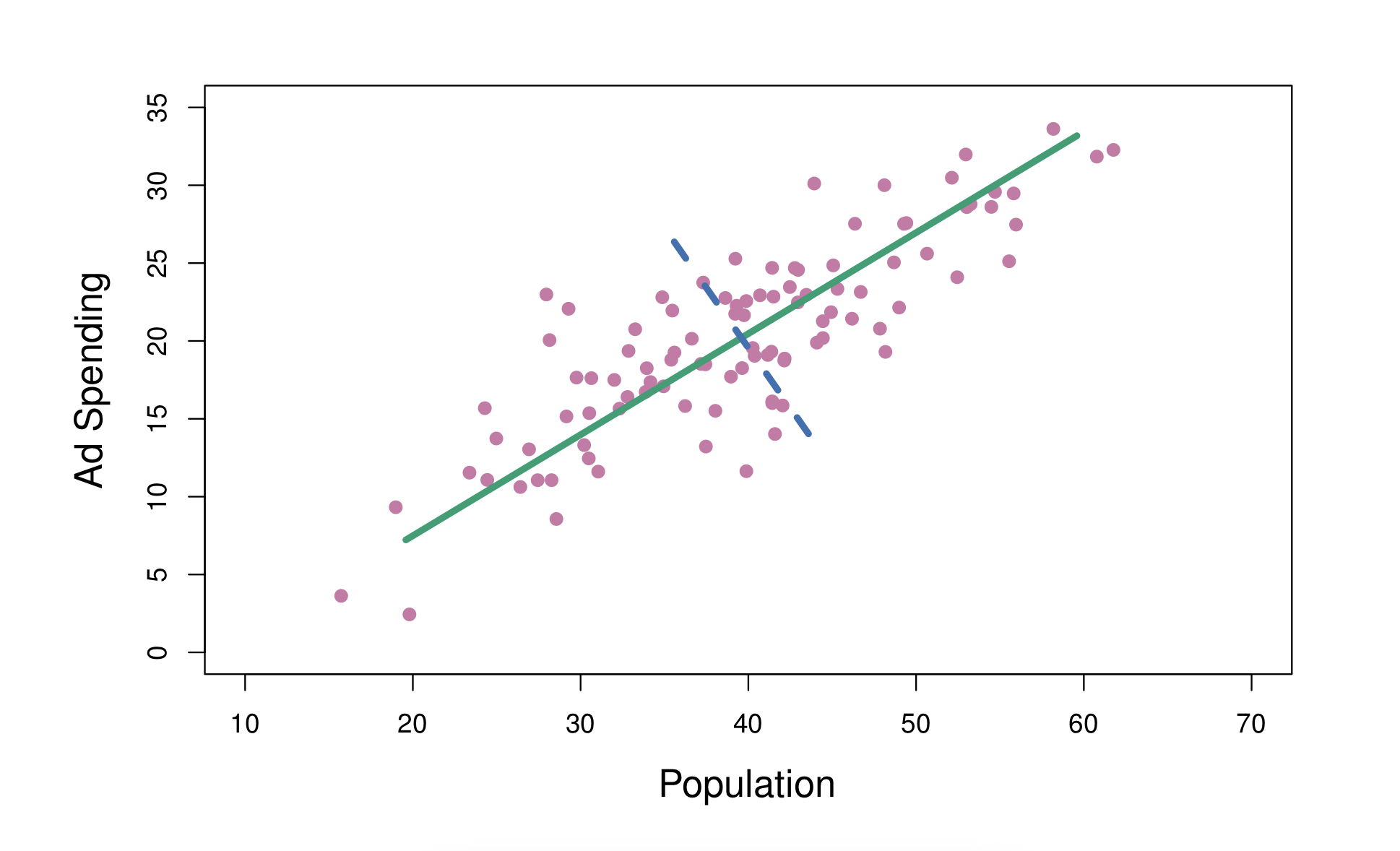
Source: James, G., Witten, D., Hastie, T., & Tibshirani, R. (2021). An Introduction to Statistical Learning: With Applications in R (2nd ed.), Figure 6.14, p. 253. Book website.

Matrix view

For centered $X$ and unit vector $w$, the projection $z = Xw$ has variance proportional to $w^\top X^\top X w$, so

$$w_1 = \arg\max_{\|w\|=1} w^\top X^\top X w$$

Using a Lagrange multiplier, this leads to

$$ X^\top X w = \lambda w. $$

Thus, $w_1$ is the eigenvector of $X^\top X$ associated with the largest eigenvalue.
The first principal component scores are

$$ z_1 = X w_1. $$

More generally, the $k$-th principal component loading vector $w_k$ is the eigenvector corresponding to the $k$-th largest eigenvalue, with orthogonality to previous components.

Interpretation

Each principal component is a weighted average of the original predictors.

• Loadings show how strongly each variable contributes to a component.
• Scores show the value of that component for each observation.

In macroeconomics, principal components are often interpreted as broad latent forces such as overall activity, financial conditions, or inflation pressure.

PCA for forecasting

Step 1: Apply PCA to $X$ and keep the first $K$ components:

$$ F_t = (F_{1t}, F_{2t}, \dots, F_{Kt})^\top. $$

Step 2: regress the future target on them:

$$ y_{t+h} = \beta_0 + \beta^\top F_t + \varepsilon_{t+h}. $$

The limitation: PCA is unsupervised — it never looks at $y$. Directions that explain $X$ are not necessarily the ones that predict $y$.

# ==================================================
# 5. PCA regression
#    PCA on indicators only, then add y_t separately
# ==================================================
X_train_ind = X_train[indicator_cols].copy()
X_test_ind = X_test[indicator_cols].copy()

scaler_pca = StandardScaler()
X_train_ind_scaled = scaler_pca.fit_transform(X_train_ind)
X_test_ind_scaled = scaler_pca.transform(X_test_ind)

# Inspect cumulative explained variance
pca_full = PCA().fit(X_train_ind_scaled)
explained_variance = np.cumsum(pca_full.explained_variance_ratio_)

plt.figure(figsize=(6, 4))
plt.plot(range(1, len(explained_variance) + 1), explained_variance, marker="o")
plt.axhline(0.8, linestyle="--")
plt.axhline(0.9, linestyle="--")
plt.xlabel("Number of Components")
plt.ylabel("Cumulative Explained Variance")
plt.title("PCA Explained Variance (Training Sample)")
plt.tight_layout()
plt.show()

Two questions for the above figure:

How many components explain 80–90% of predictor variation?

Only a few — the predictors were built from a small number of latent factors.

Are those the best components for forecasting?

Not necessarily. Explaining variation in $X$ is not the same as carrying information about $y$.

# Choose number of PCA components
n_pca = 5
n_pca = min(n_pca, X_train_ind.shape[1], X_train_ind.shape[0])

pca = PCA(n_components=n_pca)
X_train_pca = pca.fit_transform(X_train_ind_scaled)
X_test_pca = pca.transform(X_test_ind_scaled)

# Add current target y_t as an extra regressor
X_train_pca_reg = np.column_stack([X_train["y_t"].to_numpy(), X_train_pca])
X_test_pca_reg = np.column_stack([X_test["y_t"].to_numpy(), X_test_pca])

pca_reg = LinearRegression()
pca_reg.fit(X_train_pca_reg, y_train)
y_pred_pca = pca_reg.predict(X_test_pca_reg)

rmse_pca, mae_pca, r2_pca, r2_os_pca = evaluate_forecast(y_test, y_pred_pca, y_train)

print("\nOne-step-ahead PCA Regression (+ y_t)")
print("RMSE :", rmse_pca)
print("MAE  :", mae_pca)
print("R^2  :", r2_pca)
print("R^2_OS:", r2_os_pca)

One-step-ahead PCA Regression (+ y_t)
RMSE : 0.7686984158719011
MAE  : 0.5921239725364821
R^2  : 0.8035197938180847
R^2_OS: 0.8043617807628639

4. Partial Least Squares

PLS is a supervised dimension reduction method: it builds components from the predictors while also using information from the response.

Similarly, PLS constructs components as linear combinations of the predictors:

$$t_k = X w_k$$

Objective

$$w_1 = \arg\max_{\|w\|=1} \operatorname{Cov}^2(Xw, y) = \arg\max_{\|w\|=1} (w^\top X^\top y)^2$$

It picks the direction whose component is most strongly associated with the target.

PLS vs PCA

$$w_1^{\text{PCA}} = \arg\max_{\|w\|=1} w^\top X^\top X w \qquad w_1^{\text{PLS}} = \arg\max_{\|w\|=1} (w^\top X^\top y)^2$$

PCA explains variation in $X$; PLS finds directions in $X$ that predict $y$.

So PCA is unsupervised, while PLS is supervised.

Deflation

After extracting a component, PLS removes the variation it explains and repeats on the residuals. This is called deflation.

For component $k$, we work with residual matrices $X_{k-1}$ and $y_{k-1}$, and construct

$$ t_k = X_{k-1} w_k. $$

Then we write

$$ X_{k-1} = t_k p_k^\top + E_k, $$$$ y_{k-1} = t_k q_k + f_k. $$

This process continues until we keep $K$ components.

Forecasting

$$y_{t+1} = \alpha_0 + \alpha^\top t_t + \varepsilon_{t+1}$$

Extract a few supervised components, then regress the future target on them. $t_t$ is the vector of PLS component scores for observation $t$.

# ==================================================
# 6. PLS regression
#    PLS on indicators only, then add y_t separately
# ==================================================
n_pls = 5
n_pls = min(n_pls, X_train_ind.shape[1], X_train_ind.shape[0] - 1)

scaler_pls = StandardScaler()
X_train_ind_scaled = scaler_pls.fit_transform(X_train_ind)
X_test_ind_scaled = scaler_pls.transform(X_test_ind)

pls_model = PLSRegression(n_components=n_pls, scale=False)
pls_model.fit(X_train_ind_scaled, y_train)

# Extract PLS component scores
X_train_pls_scores = pls_model.transform(X_train_ind_scaled)
X_test_pls_scores = pls_model.transform(X_test_ind_scaled)

# Add current target y_t separately
X_train_pls_reg = np.column_stack([X_train["y_t"].to_numpy(), X_train_pls_scores])
X_test_pls_reg = np.column_stack([X_test["y_t"].to_numpy(), X_test_pls_scores])

pls_reg = LinearRegression()
pls_reg.fit(X_train_pls_reg, y_train)
y_pred_pls = pls_reg.predict(X_test_pls_reg)

rmse_pls, mae_pls, r2_pls, r2_os_pls = evaluate_forecast(y_test, y_pred_pls, y_train)

print("\nOne-step-ahead PLS Regression (+ y_t)")
print("RMSE :", rmse_pls)
print("MAE  :", mae_pls)
print("R^2  :", r2_pls)
print("R^2_OS:", r2_os_pls)

One-step-ahead PLS Regression (+ y_t)
RMSE : 0.8408547900696621
MAE  : 0.6706729560493282
R^2  : 0.7649020521870162
R^2_OS: 0.7659095297678349

Why can PLS lose to PCA?

Because it uses $y$ to build the components, PLS can fit noise in the training sample. PCA is less targeted but often more stable out of sample — when the main common variation in $X$ is what actually matters.

5. Sparse regression with Lasso

Motivation for sparse regression:

With a very large predictor set, it is more plausible that a small subset carries most of the signal than that every variable matters equally.

Lasso — Least Absolute Shrinkage and Selection Operator:

$$\min_{\beta_0,\beta} \left\{ \sum_{t=1}^T \left(y_{t+h}-\beta_0-x_t^\top\beta\right)^2 + \lambda \sum_{j=1}^p |\beta_j| \right\}$$

The first term is the usual fit term: it rewards the model for matching the data well.
The second term is the L1 penalty, which penalizes large absolute coefficient values.

Intuition

Lasso balances two goals:

• fit the data well
• keep the model simple

If $\lambda = 0$, Lasso reduces to ordinary least squares.
If $\lambda$ becomes larger, the penalty becomes stronger, and more coefficients are pulled toward zero.

Why it selects variables. The geometry of the L1 ball makes corner solutions likely, so the optimizer sets many $\hat{\beta}_j$ to exactly zero — automatic variable selection.

Source: Nicoguaro (2017), L1 and L2 balls, Wikimedia Commons. Licensed under CC BY 4.0.

Here, $\lambda \ge 0$ is a tuning parameter that controls the tradeoff between fit and sparsity.

• small $\lambda$: weak penalty, more coefficients kept in the model
• large $\lambda$: strong penalty, more coefficients shrunk to zero

So choosing $\lambda$ is very important. In practice, it is often selected by cross-validation or another validation procedure.

Workflow: standardize → choose $\lambda$ → estimate → forecast $\hat y_{t+1} = \hat\beta_0 + x_t^\top \hat\beta$.

Weaknesses

• results hinge on $\lambda$
• among correlated predictors it picks one and drops the rest somewhat arbitrarily
• if the truth isn't sparse, it throws away useful information
• still linear unless you add nonlinear features yourself

# ==================================================
# 7. Lasso regression with time-series CV
# ==================================================
tscv = TimeSeriesSplit(n_splits=5)

lasso_pipe = Pipeline([
    ("scaler", StandardScaler()),
    ("model", LassoCV(cv=tscv, random_state=42, max_iter=20000))
])

lasso_pipe.fit(X_train, y_train)
y_pred_lasso = lasso_pipe.predict(X_test)

rmse_lasso, mae_lasso, r2_lasso, r2_os_lasso = evaluate_forecast(
    y_test, y_pred_lasso, y_train
)

print("\nOne-step-ahead Lasso Regression")
print("RMSE :", rmse_lasso)
print("MAE  :", mae_lasso)
print("R^2  :", r2_lasso)
print("R^2_OS:", r2_os_lasso)

lasso_model = lasso_pipe.named_steps["model"]
lasso_selected_mask = lasso_model.coef_ != 0
lasso_selected_count = np.sum(lasso_selected_mask)

print("Chosen alpha:", lasso_model.alpha_)
print("Number of selected predictors:", lasso_selected_count)

selected_predictors = X_train.columns[lasso_selected_mask]
print("Selected predictors:")
print(list(selected_predictors))

selected_features = pd.Series(lasso_model.coef_, index=X_train.columns)
selected_features = selected_features[selected_features != 0].sort_values(
    key=np.abs, ascending=False
)

print("\nTop selected features:")
print(selected_features.head(10))

One-step-ahead Lasso Regression
RMSE : 0.8052663679011026
MAE  : 0.6472958655221215
R^2  : 0.784381532389933
R^2_OS: 0.7853055335313653
Chosen alpha: 0.12994408894406342
Number of selected predictors: 5
Selected predictors:
['indicator_14', 'indicator_15', 'indicator_34', 'indicator_40', 'y_t']

Top selected features:
y_t             0.648329
indicator_15    0.270106
indicator_40   -0.153188
indicator_34    0.108117
indicator_14    0.080035
dtype: float64

Interpretation of the results

Lasso roughly matches AR(1) — RMSE, MAE and out-of-sample $R^2$ all close, but not better. Most predictive power sits in a few variables, not in all 60.

How many predictors did Lasso keep? Five: indicator_14, indicator_15, indicator_34, indicator_40, and y_t.

Does selection help interpretability? Yes — a handful of nonzero coefficients makes it obvious that $y_t$ dominates and only a few indicators add signal.

Small subset or broad co-movement? Depends on the goal. Selection buys interpretability and stability; factor methods win when many variables genuinely share common information. In macro data both have a place.

6. Neural networks

A neural network is a flexible prediction model that learns a nonlinear relationship between the predictors and the response:

$$ y_{t+1} = f(x_t) + \varepsilon_{t+1}, $$

where $f(\cdot)$ is a nonlinear function learned from the data.

One-hidden-layer neural network

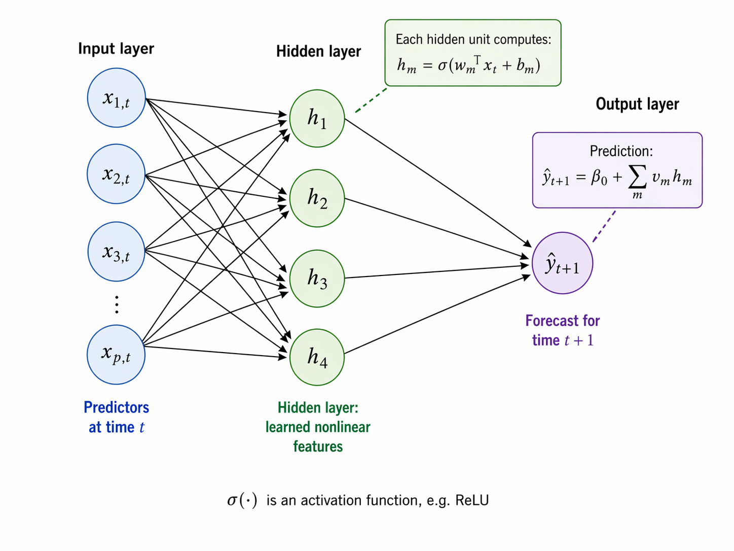
Source: Generated by Chatgpt.

A simple feedforward neural network with one hidden layer can be written as

$$y_{t+1} = \beta_0 + \sum_{m=1}^M v_m \, \sigma(w_m^\top x_t + b_m) + \varepsilon_{t+1}$$

where:

• $M$ is the number of hidden units,
• $w_m \in \mathbb{R}^p$ is the weight vector for hidden unit $m$,
• $b_m$ is the bias term for hidden unit $m$,
• $v_m$ is the weight from hidden unit $m$ to the output,
• $\sigma(\cdot)$ is an activation function.

Each hidden unit takes a linear combination $a_m = w_m^\top x_t + b_m$, applies a nonlinearity $h_m = \sigma(a_m)$; the output is a weighted sum of those units.

Activation functions

The activation function introduces nonlinearity into the model.

A common example is the ReLU activation:

$$ \sigma(a) = \max(0, a). $$

Without a nonlinear activation the whole network collapses to a linear model.

Compact form

$$h_t = \sigma(W x_t + b), \qquad \hat{y}_{t+1} = \beta_0 + v^\top h_t$$

The network first learns a representation of the predictors, then forecasts from it.

Deeper networks stack the step:

$$h_t^{(1)} = \sigma(W^{(1)} x_t + b^{(1)}), \quad h_t^{(2)} = \sigma(W^{(2)} h_t^{(1)} + b^{(2)}), \quad \dots$$

which is why these are called representation learning methods: they learn increasingly abstract transformations of the predictors.

Estimation

Neural networks are usually estimated by minimizing a loss function, such as mean squared error in regression:

$$ \min_{\theta} \sum_t \left(y_{t+1} - \hat{y}_{t+1}\right)^2, $$

where $\theta$ represents all network parameters: weights, biases, and output coefficients.

No closed form — gradient descent and its variants.

Limitations

Harder to interpret · sensitive to tuning · computationally heavier · prone to overfitting in small samples.

In macro settings they do not automatically beat simpler methods. Treat them as a flexible benchmark, not a default.

# ==================================================
# 8. Neural network
# ==================================================
mlp_pipe = Pipeline([
    ("scaler", StandardScaler()),
    ("model", MLPRegressor(
        hidden_layer_sizes=(32, 16),
        activation="relu",
        alpha=0.001,
        max_iter=3000,
        random_state=42
    ))
])

mlp_pipe.fit(X_train, y_train)
y_pred_mlp = mlp_pipe.predict(X_test)

rmse_mlp, mae_mlp, r2_mlp, r2_os_mlp = evaluate_forecast(y_test, y_pred_mlp, y_train)

print("\nOne-step-ahead Neural Network")
print("RMSE :", rmse_mlp)
print("MAE  :", mae_mlp)
print("R^2  :", r2_mlp)
print("R^2_OS:", r2_os_mlp)

One-step-ahead Neural Network
RMSE : 0.9772225673080337
MAE  : 0.8045075750652662
R^2  : 0.6824633867086518
R^2_OS: 0.6838241430315211

7. Comparing the methods

No method wins everywhere. Compare on out-of-sample performance, interpretability, stability, computational cost, and fit to the research question.

# ==================================================
# 9. Collect results
# ==================================================
results = pd.DataFrame({
    "Model": [
        "AR(1)",
        "Linear Regression",
        "PCA Regression",
        "PLS Regression",
        "Lasso",
        "Neural Network"
    ],
    "RMSE": [
        rmse_ar,
        rmse_baseline,
        rmse_pca,
        rmse_pls,
        rmse_lasso,
        rmse_mlp
    ],
    "MAE": [
        mae_ar,
        mae_baseline,
        mae_pca,
        mae_pls,
        mae_lasso,
        mae_mlp
    ],
    "R2_sklearn": [
        r2_ar,
        r2_baseline,
        r2_pca,
        r2_pls,
        r2_lasso,
        r2_mlp
    ],
    "R2_OS": [
        r2_os_ar,
        r2_os_baseline,
        r2_os_pca,
        r2_os_pls,
        r2_os_lasso,
        r2_os_mlp
    ],
    "Extra": [
        "Uses y_t only",
        "Uses all indicators + y_t",
        f"{n_pca} PCA comps + y_t",
        f"{n_pls} PLS comps + y_t",
        f"alpha={lasso_model.alpha_:.4f}, selected={lasso_selected_count}",
        "MLP(32,16)"
    ]
})

results = results.sort_values("RMSE").reset_index(drop=True)

print("\nFull comparison table:")
print(results)


# ==================================================
# 10. RMSE comparison
# ==================================================
plt.figure(figsize=(5, 3))
plt.bar(results["Model"], results["RMSE"])
plt.xticks(rotation=30, ha="right")
plt.ylabel("RMSE")
plt.title("One-step-ahead Forecast Comparison by RMSE")
plt.tight_layout()
plt.show()


# ==================================================
# 11. Out-of-sample R^2 comparison
# ==================================================
plt.figure(figsize=(5, 3))
plt.bar(results["Model"], results["R2_OS"])
plt.axhline(0, linestyle="--")
plt.xticks(rotation=30, ha="right")
plt.ylabel("Out-of-sample $R^2$")
plt.title("One-step-ahead Forecast Comparison by Out-of-sample $R^2$")
plt.tight_layout()
plt.show()


# ==================================================
# 12. Predicted vs actual values
# ==================================================
pred_df = pd.DataFrame({
    "Actual": y_test.values,
    "AR(1)": y_pred_ar,
    "Linear": y_pred_baseline,
    "PCA": y_pred_pca,
    "PLS": y_pred_pls,
    "Lasso": y_pred_lasso,
    "NeuralNet": y_pred_mlp,
    "BenchmarkMean": np.repeat(y_train.mean(), len(y_test))
}, index=y_test.index)

plt.figure(figsize=(6, 3))
plt.plot(pred_df.index, pred_df["Actual"], label="Actual")
plt.plot(pred_df.index, pred_df["AR(1)"], label="AR(1)")
plt.plot(pred_df.index, pred_df["PCA"], label="PCA")
plt.plot(pred_df.index, pred_df["PLS"], label="PLS")
plt.plot(pred_df.index, pred_df["Lasso"], label="Lasso")
plt.plot(pred_df.index, pred_df["BenchmarkMean"], label="Benchmark Mean")
plt.legend()
plt.title("Actual vs Predicted Values (One-step-ahead Forecasts)")
plt.tight_layout()
plt.show()


# ==================================================
# 13. Rounded summary table
# ==================================================
results_display = results.copy()
for col in ["RMSE", "MAE", "R2_sklearn", "R2_OS"]:
    results_display[col] = results_display[col].round(3)

print("\nRounded comparison table:")
print(results_display)

Full comparison table:
               Model      RMSE       MAE  R2_sklearn     R2_OS  \
0     PCA Regression  0.768698  0.592124    0.803520  0.804362   
1              AR(1)  0.801646  0.640657    0.786316  0.787232   
2              Lasso  0.805266  0.647296    0.784382  0.785306   
3     PLS Regression  0.840855  0.670673    0.764902  0.765910   
4  Linear Regression  0.917795  0.764769    0.719909  0.721110   
5     Neural Network  0.977223  0.804508    0.682463  0.683824   

                       Extra  
0          5 PCA comps + y_t  
1              Uses y_t only  
2   alpha=0.1299, selected=5  
3          5 PLS comps + y_t  
4  Uses all indicators + y_t  
5                 MLP(32,16)  

Rounded comparison table:
               Model   RMSE    MAE  R2_sklearn  R2_OS  \
0     PCA Regression  0.769  0.592       0.804  0.804   
1              AR(1)  0.802  0.641       0.786  0.787   
2              Lasso  0.805  0.647       0.784  0.785   
3     PLS Regression  0.841  0.671       0.765  0.766   
4  Linear Regression  0.918  0.765       0.720  0.721   
5     Neural Network  0.977  0.805       0.682  0.684   

                       Extra  
0          5 PCA comps + y_t  
1              Uses y_t only  
2   alpha=0.1299, selected=5  
3          5 PLS comps + y_t  
4  Uses all indicators + y_t  
5                 MLP(32,16)  

Results

PCA regression wins — lowest RMSE and MAE, highest out-of-sample $R^2$. Summarizing the predictors into a few common components works well when the data really was generated by common factors.

AR(1) and Lasso come next and are close to each other: target persistence matters a lot, and a small sparse set captures most of the remaining signal.

PLS is respectable but doesn't beat PCA — supervised components overfit the training sample here.

Full OLS and the neural network trail. Using all predictors directly hurts in high dimensions, and the network doesn't recover enough nonlinear structure to justify its flexibility.

8. Which method, when?

PCA / factor models — predictors strongly correlated, common latent structure plausible, you want stable low-dimensional summaries, co-movement is the point.

PLS — prediction is the goal, predictors many and correlated, you want the reduction to be supervised.

Lasso — interpretability matters, many predictors are probably irrelevant, a sparse model is desirable.

Neural networks — nonlinear structure matters, data is plentiful, and the flexibility is worth the complexity.